Preamble

This is the first post in a series looking back at past projects I have done but not shared publicly or documented in any way.

This was a piece of work from 2019 with the goal of extracting road markings from geo-referenced pointclouds. For those that don’t know, a geo-referenced pointcloud is created by taking a LiDAR and putting it on some kind of a rover vehicle, then taking all the observations of the LiDAR that were taken in the moving vehicle reference frame and converting them into the global “static” reference frame. To do this you need to have accurate estimation of the rover vehicle’s six degree of freedom position and orientation, as well as the six degree of freedom translation and rotation between the LiDAR origin and navigation origin. Calibrating these two sensor origins accurately is enough to write a white paper on so I won’t cover it here, but suffice to say that CAD models and accurate manufacturing of mounts is not good enough when the LiDAR range to target is over a few metres.

A car was instrumented with an OxTS xNAV550 (now superseded by the xNAV650) inertial navigation system and Velodyne VLP-16 (now branded as the Puck) LiDAR. Both systems were calibrated and then a range of sorties were conducted driving on open roads and private vehicle proving grounds.

The data from these runs was then taken and processed to provide accurate, geo-referenced positions of simplified representations of any observed road markings. These representations can then be used for development and validation of advanced driver assistance systems (ADAS) and autonomous vehicle functions.

The following post describes the processing approach that was used and provides some results comparing this method of instrumentation and processing versus a traditional RTK GNSS survey approach.

Typical Input

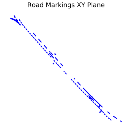
I thought it would be useful to take a quick look at a couple of typical geo-referenced pointclouds used as input. Figure 1 shows one of the simpler cases taken from a straight section of an automotive proving ground. The points are coloured black to white according to the reflectance value of the point return recorded by the LiDAR. The road markings record high reflectance values as they are designed to be seen clearly by vehicles headlights, we can leverage this later.

Figure 1: Simple Case

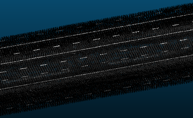
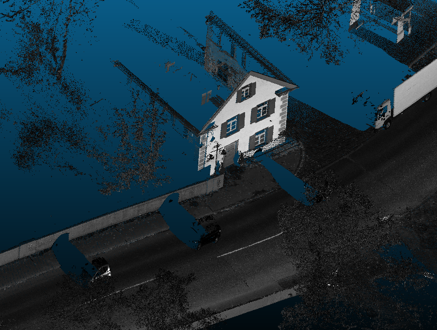
Figure 2 shows a more complex case. This dataset was taken on a section of public road. Here there are a great deal more observations further from the road surface. You can see buildings and trees, as well as other roadside furniture.

Figure 2: Complex Case

Extracting The Road/Ground Points

Roads tend to lay on the ground and even when they don’t they tend to form a pretty good approximation of a 2D plane. Roads do tend to have some curvature across them to allow for curb side drainage of rain water but we can account for this.

I used a technique called Random Sample Consensus (RANSAC) to fit a plane to the complete pointcloud data set. If I had used RMSE to fit the plane it would rarely lie on the road due to the other features (buildings, trees, etc.) within the pointcloud. Functions like RMSE weight all points equally, whereas we need to consider any points not on the road surface as noise. RANSAC allows us to iteratively try a number of different fits for our plane and score each iteration based on how many points lie within a predefined margin of error around the plane, then we simply use the best one. To better illustrate how RANSAC works I always point people to this page from the Scikit-Learn documentation.

The margin of error we define for the RANSAC regressor can be the vertical deviation of the road surface mentioned earlier. On multiple occasions we’ll use similar priors about the environment to help us leverage various unsupervised machine learning methods. This is great as it allows us to arrive at a solution without the time intensive data collection and labeling required in supervised learning approaches. At the time of writing there are significantly more open source labeled data sets available but in 2019 there wasn’t a great deal of accurate annotated ope source pointcloud data sets.

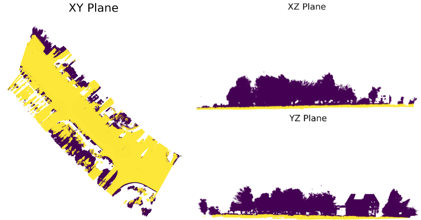
Figure 3 shows the points fitted to the ground plane in yellow and the excluded points in purple. You can clearly see the separation of LiDAR observations lying on the ground and those on trees and buildings.

Figure 3: RANSAC Ground Extraction

Filter on Intensity

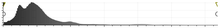
As can be seen in figures 1 and 2 the reflectance intensity values of the road markings and the asphalt are very different. Figure 4 shows the distribution of intensities for the complex case (figure 2). Some manual analysis of your input data will let you determine a reflectance intensity band in which the road markings lie. This can be used to apply thresholds to remove all points that do not closely match the reflectance of the lane markings. These values will not be universal though as different sensors and environments may yield different results.

Figure 4: Reflectance Intensity Distribution

It can also be useful to apply some filtering at this stage to clean up what we have left. DBSCAN (Density-Based Spatial Clustering of Applications with Noise) is perfect for this, though it is usually used as a powerful clustering algorithm, we can use it to disregard points that are a given Euclidean distance away from our main clusters of points, leaving us with the high reflectance points lying within the ground plane (figure 5).

Figure 5: Pointcloud of Extracted Road Markings

This may be enough for some applications but we’ll press on and see if we can get to a simplified line representation of the lane lines.

Adapted K-Means Clustering Using Parallel Lines as Centroids

K-Means clustering is one of the most commonly used clustering algorithms in spite of it’s many drawbacks.

Normally in k-means clustering we:

set a value for “k”, the number of clusters in your data set
randomly generate the position for the centroid of these clusters
group all the data points by which centroid they are closest to
compute a new centroid as the mean position for each cluster group
repeat steps 3 and 4 until you converge on a solution

Here I decided to use an adapted version of this algorithm where the centroids were parallel lines rather than points. Clearly parallel lines only works on particular road markings and would struggle with curvature, but the though here was that it would be possible to discretise many curved lane markings into a series of straight lines, this would be even more viable if the process was to run in “real-time” as the instrumented vehicle surveys the road.

In the adapted algorithm we:

establish the direction of the road (m value in y=mx+c) using a RANSAC line fitment to the pointcloud of road markings on the ground
set a value for “k”, this should be the number of lane lines in the data set
create “k” parallel lines with a gradient equal to the line in 1. and offset (c value in y=mx+c) from each other by around 3 metres (this is the typical distance between road lane markings)
group all the data points by which line they are closest to
compute a new the line for each cluster group
use the new lines offset (c value in y=mx+c) and keep the gradient (m value in y=mx+c) from the line in 1. and combine these to give a new line to be used as the cluster centre
repeat steps 4 through 6 until you converge on a solution

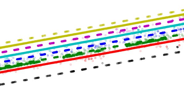
The output from this can be seen in figure 6 where the clusters are coloured differently in each identified group.

Figure 6: Individiual Lane Clusters

We could use the final centroid parallel lines as our final simplified lane line representation but I thought taking one additional step would help capture any lack of parallelism in the real lines.

RANSAC Simplified Line Representation

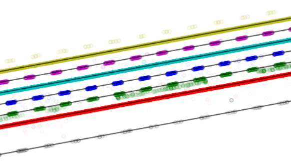
Finally we can use RANSAC once again, this time on each separate cluster of points to provide our final simplified line representation of the set of lanes. Figure 7 shows these lines overlayed on the clustered lane marking points used to create them.

Figure 7: Clustered and Simplified

Results

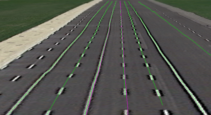
We can make a comparison with aerial imagery, provided here by Google Earth, in figure 8. The green lines in the figure are those generated by the processing method given here, whereas the magenta line was created using an RTK GNSS survey of the right hand side of the lane marking it lies on.

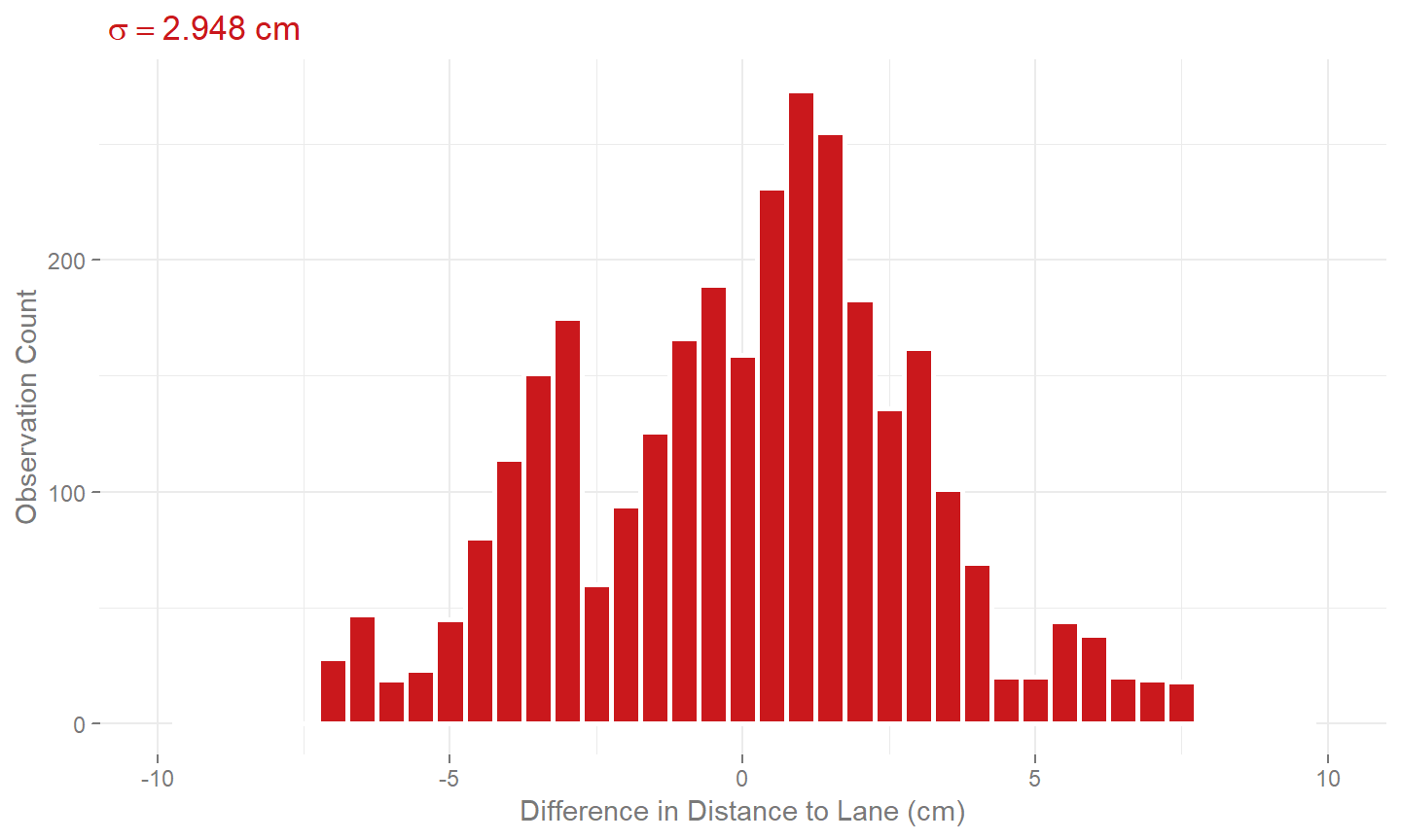
Figure 8: Aerial Photo with Line Overlay

We can benchmark a comparison of the lanes created here and those created using an RTK GNSS survey. Rather than just comparing the position of the lines with each other, it was decided to drive through the lanes using the instrumented vehicle and computing the lateral distance to both lines. The difference in the lateral distances between the RTK GNSS surveyed line and the vehicle, and the LiDAR surveyed line and the vehicle are provided in figure 9. This was done partly because establishing absolute accuracy is hard and establishing relative performance versus the traditionally used alternative is easier and in some ways more practical. I wouldn’t claim that using a LiDAR and RTK INS on a vehicle to remotely sense the position of lanes marking would be more accurate than directly using RTK GNSS, but one is much more time intensive than the other. Walking around with a survey pole can take days to cover a site and may not be practical on a public highway. Using a drive-by remote method can greatly increase the speed of data capture if the trade off in accuracy is allowable.

Figure 9: Error vs. Traditional GNSS Survey

Further Development

As with everything in life, once you finish up with something you can think of a slew of ways you could have done it better. Here are some ideas for what to do to improve upon the process outlines here.

fit a shape envelope to each marking to reduce noise points (use of prior knowledge of the lane geometry)
cluster and line fitment for each individual marking and use principle component analysis to determine orientation each road marking’s orientation
extension to capture lane curvature with time segmentation and poly-line fitment

Extracting Road Markings from Pointcloud Data