Preamble

Registration is the technique of aligning two data sets by finding either a rigid or affine transformation, depending on the problem. In robotics this is often between two pointclouds but the technique can be useful for aligning any data sets especially those that contain spatial data, MRI scan images for example. The Wikipedia page for this topic is quite concise and well written.

Background

Typically we represent transformations in 3D space as a matrix and translation vector that we apply to an input vector of coordinates to produce a transformed output vector of shifted coordinates. \[\begin{equation} \begin{bmatrix} a & b & c\\ d & e & f\\ g & h & i \end{bmatrix} \begin{bmatrix} x_{in}\\ y_{in}\\ z_{in} \end{bmatrix} + \begin{bmatrix} t_x\\ t_y\\ t_z \end{bmatrix} = \begin{bmatrix} x_{out}\\ y_{out}\\ z_{out} \end{bmatrix} \tag{1} \end{equation}\]

The matrix can perform a variety of operations all at once, rotation, shearing, scaling and mirroring. If we have a given transformation matrix there are some operations we can do to see what the output is likely to be.

If the norm for each column vector inside the transformation matrix are equal to each other and one then there is no scaling and we lose three degrees of freedom. \[\begin{equation} ||V_1|| = (a^2 + d^2 + g^2)^{-0.5} \end{equation}\]

\[\begin{equation} ||V_2|| = (b^2 + e^2 + h^2)^{-0.5} \end{equation}\]

\[\begin{equation} ||V_3|| = (c^2 + f^2 + i^2)^{-0.5} \end{equation}\]

\[\begin{equation} ||V_1|| = ||V_2|| = ||V_3|| = 1 \end{equation}\]

If the dot product of each of the three combinations of pairs of column vectors equal zero, then there is no shearing and we lose another three degrees of freedom. \[\begin{equation} \begin{bmatrix} a\\ d\\ g \end{bmatrix} \cdot \begin{bmatrix} b\\ e\\ h \end{bmatrix} = 0 \end{equation}\]

\[\begin{equation} \begin{bmatrix} a\\ d\\ g \end{bmatrix} \cdot \begin{bmatrix} c\\ f\\ i \end{bmatrix} = 0 \end{equation}\]

\[\begin{equation} \begin{bmatrix} b\\ e\\ h \end{bmatrix} \cdot \begin{bmatrix} c\\ f\\ i \end{bmatrix} = 0 \end{equation}\]

If we calculate the determinant of the transformation matrix and it is positive then the solution is not mirrored, where as if it is negative then the output will be mirrored. \[\begin{equation} \begin{vmatrix} a & b & c\\ d & e & f\\ g & h & i \end{vmatrix} = 1 \end{equation}\]

\[\begin{equation} \begin{vmatrix} a & b & c\\ d & e & f\\ g & h & i \end{vmatrix} = -1 \end{equation}\]

Finally, if our matrix is actually the identity matrix then there is no transformation applied by the matrix. \[\begin{equation} \begin{bmatrix} a & b & c\\ d & e & f\\ g & h & i \end{bmatrix} = \begin{bmatrix} 1 & 0 & 0\\ 0 & 1 & 0\\ 0 & 0 & 1 \end{bmatrix} \end{equation}\]

Homogeneous Coordinates

It can often be useful to represent transformation operations in homogeneous coordinates by adding an additional dimension to all the members to facilitate a single operation. \[\begin{equation} \begin{bmatrix} a & b & c & t_x\\ d & e & f & t_y\\ g & h & i & t_z\\ 0 & 0 & 0 & 1 \end{bmatrix} \begin{bmatrix} x\\ y\\ z\\ 1 \end{bmatrix} = \begin{bmatrix} x_{ref}\\ y_{ref}\\ z_{ref}\\ 1 \end{bmatrix} \end{equation}\]

Reference Data Set

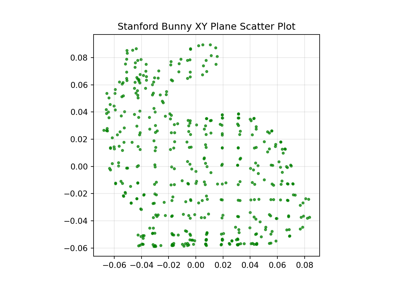
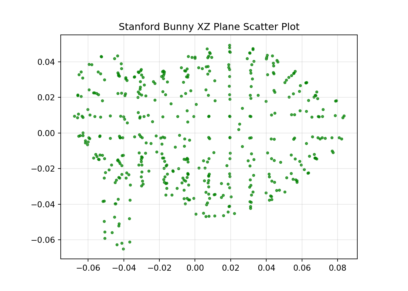
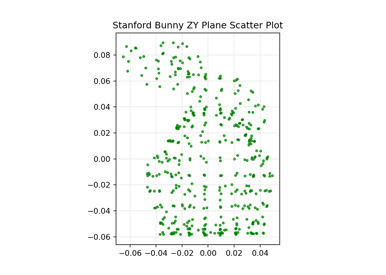
We will use a 3D point set of the Standford Bunny to take a look at some different methods of point set registration. This provides a good none homogeneous 3D data set for trying to evaluate the strengths and weaknesses of these methods.

Transformed Only Problem

Let’s start off with a simple example. We can take the original data set and apply a known transformation. Here I have rotated the bunny by 120, 75 and 21 degrees of yaw, pitch and roll respectively.

I have also translated the bunny by 0.25, -0.1 and 0.01, in x, y and z respectively.

An important note with this data set is that all the points maintain correspondence between each other, ie. the first point in both data sets relate to the same point on the bunny, as does the second and so on. This can be the case sometimes in the real world when you have some method of achieving this correspondence, like a time stamp for example.

Solution as a System of Linear Equations

If we write equation (1) in terms of the column vectors we come to the following representation.

\[\begin{equation} \begin{bmatrix} a\\ d\\ g \end{bmatrix} x + \begin{bmatrix} b\\ e\\ h \end{bmatrix} y + \begin{bmatrix} c\\ f\\ i \end{bmatrix} z + \begin{bmatrix} t_x\\ t_y\\ t_z \end{bmatrix} = \begin{bmatrix} x_{ref}\\ y_{ref}\\ z_{ref} \end{bmatrix} \end{equation}\]

If \(x\), \(y\), \(z\) and \(x_{ref}\), \(y_{ref}\), \(z_{ref}\) are all known. Then we are left with a system of three equations with twelve unknowns. In order to solve this we will need four observations. If this were the 2D case, rather than the 3D case, you would have six unknowns across two equations, requiring a minimum of three observations. Here we have assumed correspondence between our reference data and input data, as such this method will fail on our corrupted data without correspondence.

With some rearrangement we can set this system of equations up as an \(A \vec x=B\) problem with three rows in \(A\) and \(B\) for each of the three equations, then repeating for \(n\) observations. All of our twelve unknowns form the vector \(\vec x\). We can then solve as \(\vec x =A^{-1}B\) using a least squares solver to provide our transform.

\[\begin{equation} \begin{bmatrix} x_1 & y_1 & z_1 & 0 & 0 & 0 & 0 & 0 & 0 & 1 & 0 & 0\\ 0 & 0 & 0 & x_1 & y_1 & z_1 & 0 & 0 & 0 & 0 & 1 & 0\\ 0 & 0 & 0 & 0 & 0 & 0 & x_1 & y_1 & z_1 & 0 & 0 & 1\\ x_2 & y_2 & z_2 & 0 & 0 & 0 & 0 & 0 & 0 & 1 & 0 & 0\\ 0 & 0 & 0 & x_2 & y_2 & z_2 & 0 & 0 & 0 & 0 & 1 & 0\\ 0 & 0 & 0 & 0 & 0 & 0 & x_2 & y_2 & z_2 & 0 & 0 & 1\\ & & & & & ...\\ x_n & y_n & z_n & 0 & 0 & 0 & 0 & 0 & 0 & 1 & 0 & 0\\ 0 & 0 & 0 & x_n & y_n & z_n & 0 & 0 & 0 & 0 & 1 & 0\\ 0 & 0 & 0 & 0 & 0 & 0 & x_n & y_n & z_n & 0 & 0 & 1 \end{bmatrix} \begin{bmatrix} a\\ b\\ c\\ d\\ e\\ f\\ g\\ h\\ i\\ t_x\\ t_y\\ t_z \end{bmatrix} = \begin{bmatrix} x_{ref_1}\\ y_{ref_1}\\ z_{ref_1}\\ x_{ref_2}\\ y_{ref_2}\\ z_{ref_2}\\ ...\\ x_{ref_n}\\ y_{ref_n}\\ z_{ref_n} \end{bmatrix} \end{equation}\]

###################################################################################################################################
# 3D Linear Least Square Registration
###################################################################################################################################
# ref_xyz = the original reference data as an array of three columns x, y, and z with as many rows as points
# trans_xyz = the transformed data as an array of three columns x, y, and z with as many rows as points

A = np.zeros((3*len(trans_xyz), 12))
B = np.zeros((3*len(trans_xyz), 1))

for i in range(0, len(trans_xyz)-1):
     # Equation 1
     A[3*i+1, 0] = trans_xyz[i+1, 0]
     A[3*i+1, 1] = trans_xyz[i+1, 1]
     A[3*i+1, 2] = trans_xyz[i+1, 2]
     A[3*i+1, 3] = 0
     A[3*i+1, 4] = 0
     A[3*i+1, 5] = 0
     A[3*i+1, 6] = 0
     A[3*i+1, 7] = 0
     A[3*i+1, 8] = 0
     A[3*i+1, 9] = 1
     A[3*i+1, 10] = 0
     A[3*i+1, 11] = 0
     
     B[3*i+1, 0] = ref_xyz[i+1, 0]
     
     # Equation 2
     A[3*i+2, 0] = 0
     A[3*i+2, 1] = 0
     A[3*i+2, 2] = 0
     A[3*i+2, 3] = trans_xyz[i+1, 0]
     A[3*i+2, 4] = trans_xyz[i+1, 1]
     A[3*i+2, 5] = trans_xyz[i+1, 2]
     A[3*i+2, 6] = 0
     A[3*i+2, 7] = 0
     A[3*i+2, 8] = 0
     A[3*i+2, 9] = 0
     A[3*i+2, 10] = 1
     A[3*i+2, 11] = 0
     
     B[3*i+2, 0] = ref_xyz[i+1, 1]

     # Equation 3
     A[3*i+3, 0] = 0
     A[3*i+3, 1] = 0
     A[3*i+3, 2] = 0
     A[3*i+3, 3] = 0
     A[3*i+3, 4] = 0
     A[3*i+3, 5] = 0
     A[3*i+3, 6] = trans_xyz[i+1, 0]
     A[3*i+3, 7] = trans_xyz[i+1, 1]
     A[3*i+3, 8] = trans_xyz[i+1, 2]
     A[3*i+3, 9] = 0
     A[3*i+3, 10] = 0
     A[3*i+3, 11] = 1
     
     B[3*i+3, 0] = ref_xyz[i+1, 2]

# Solve
x, resid, rank, s = np.linalg.lstsq(A, B, rcond=-1)

# Compile rotation matrix
regrot = np.array([[x[0][0], x[1][0], x[2][0]],
                   [x[3][0], x[4][0], x[5][0]],
                   [x[6][0], x[7][0], x[8][0]]])

# Compile translation vector
regtrans = np.array([[x[9][0]],
                     [x[10][0]],
                     [x[11][0]]])

# Optionally check for scaling
x_scale = np.linalg.norm(regrot[:,0])
y_scale = np.linalg.norm(regrot[:,1])
z_scale = np.linalg.norm(regrot[:,2])

# Apply the computed transform for comparison
regx = regrot[0,0]*trans_xyz[:,0] + regrot[0,1]*trans_xyz[:,1] + regrot[0,2]*trans_xyz[:,2] + regtrans[0]
regy = regrot[1,0]*trans_xyz[:,0] + regrot[1,1]*trans_xyz[:,1] + regrot[1,2]*trans_xyz[:,2] + regtrans[1]
regz = regrot[2,0]*trans_xyz[:,0] + regrot[2,1]*trans_xyz[:,1] + regrot[2,2]*trans_xyz[:,2] + regtrans[2]

# Compile to one array
# reg_xyz = the transformed data registered back on to the reference data as an array of three columns x, y, and z with as many rows as points
reg_xyz = np.vstack((regx, regy, regz)).T

The results of the registration are shown below.

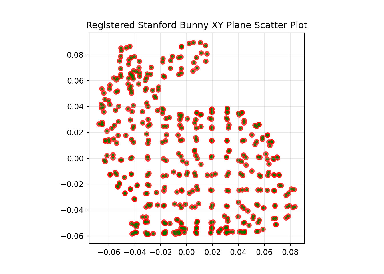
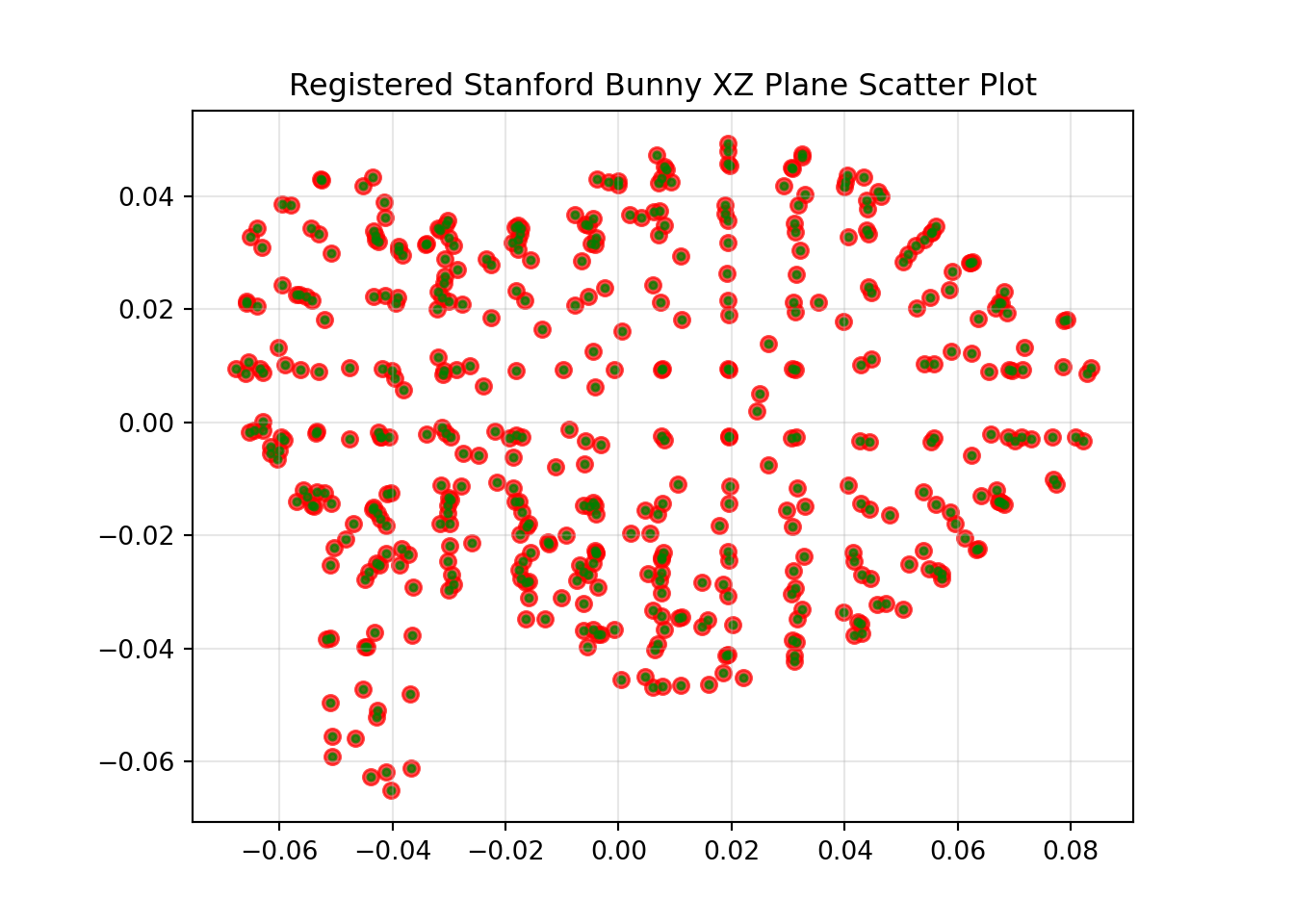
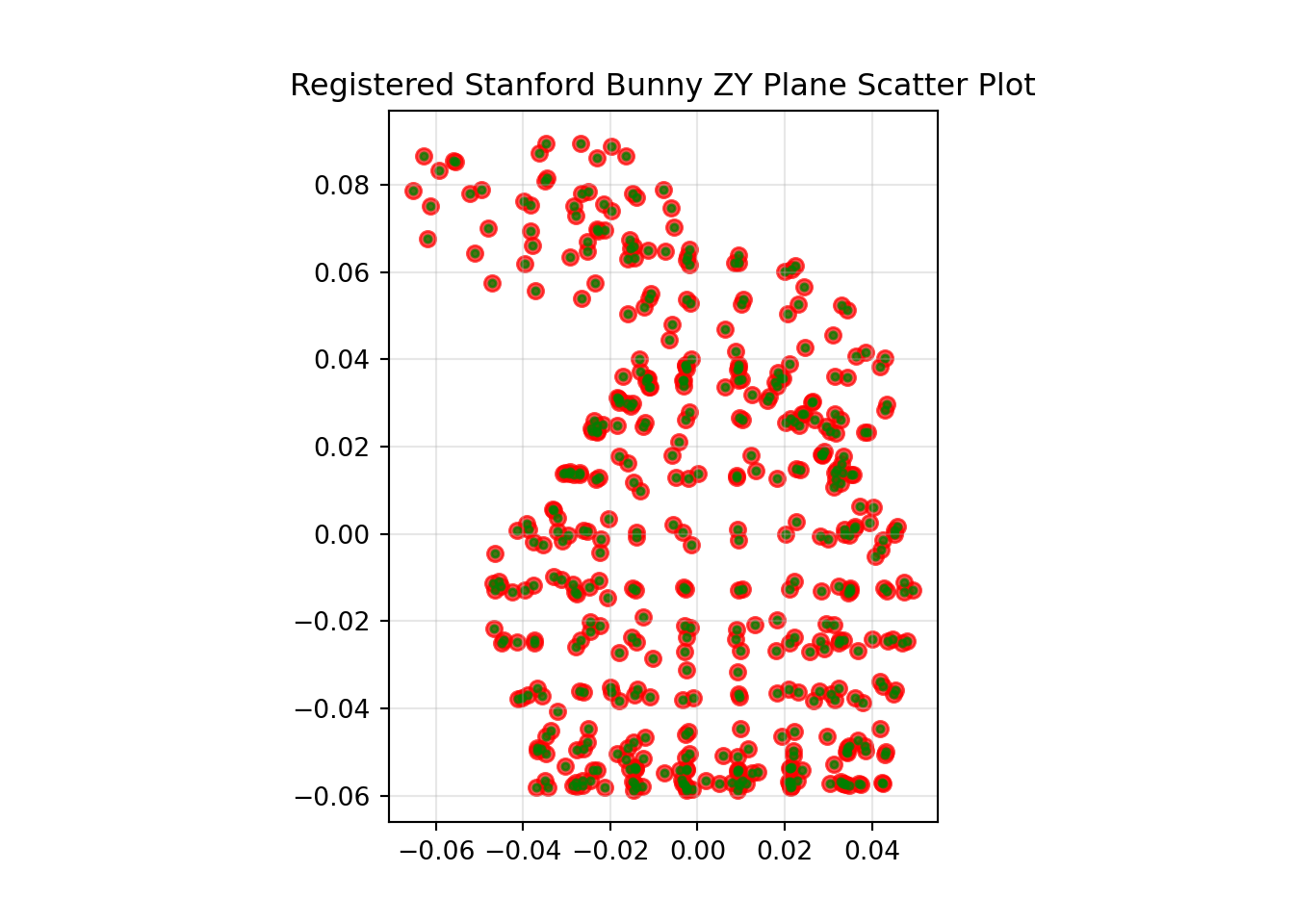
A scaling of 1 has been applied to the \(x\) axis, 1 has been applied to the \(y\) axis and 1 has been applied to the \(z\) axis.

The original transformation applied was 120, 75 and 21 degrees of yaw, pitch and roll respectively, with a translation of 0.25, -0.1 and 0.01, in x, y and z respectively.

The calculated registration transformation was 120, 75 and 21 degrees of yaw, pitch and roll respectively, with a translation of -0.064, -0.082 and 0.248, in x, y and z respectively.

Transformed and Corrupted Problem

To add some noise points to the data set I have corrupted it by taking 50 of the 453 observations and adding a random number between -0.025 and 0.025 to them.

Transformed and Corrupted Problem Without Correspondence

As a final and worst case input data set I reordered all of the points in the corrupted data set to remove the correspondence between points. If I plotted this data it would look the same as the corrupted data but the difference is purely in the row order of entries in the array.

Coherent Point Drift (CPD)

Andriy Myronenko and Xubo Song presented CPD in their paper in 2009. This work has then been implemented in a Python package by Siavash Khallaghi, who has a really useful blog post on the subject. If you want to learn the details of how it works I’d recommend visiting these links. In a nutshell it is a probabilistic approach that is resilient to noise and does not require correspondence of points. Usage with Siavash’s Python package is really straight forward.

###################################################################################################################################
# Cohernet Point Drift Registration
###################################################################################################################################
# ref_xyz = the original reference data as an array of three columns x, y, and z with as many rows as points
# shuf_corr_xyz = the transformed, corrupted and none-correspondent data as an array of three columns x, y, and z with as many rows as points

reg_type = "rigid"

# Compute CPD registration
if reg_type == "rigid":
    reg = RigidRegistration(**{ 'X': ref_xyz, 'Y': shuf_corr_xyz })
elif reg_type == "affine":
    reg = AffineRegistration(**{ 'X': ref_xyz, 'Y': shuf_corr_xyz })

reg = reg.register()

# Save array of registered points
# reg_xyz = the transformed, corrupted and none-correspondent data registered back on to the reference data as an array of three columns x, y, and z with as many rows as points
reg_xyz = reg[0]

The results of the CPD rigid registration are shown below.

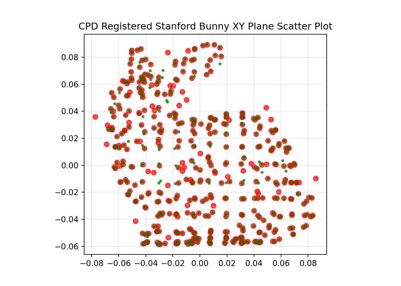
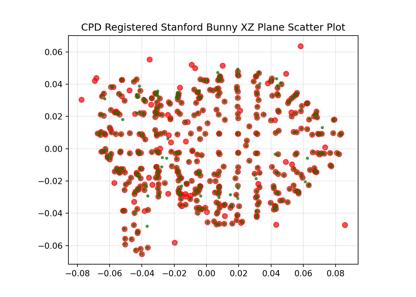
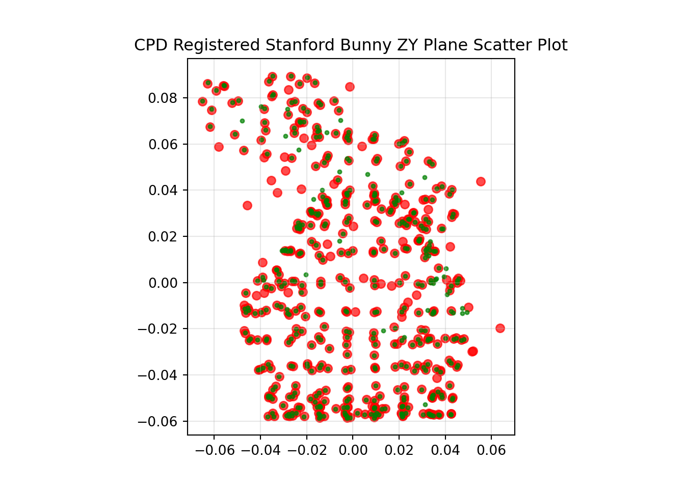
The original transformation applied was 120, 75 and 21 degrees of yaw, pitch and roll respectively, with a translation of 0.25, -0.1 and 0.01, in x, y and z respectively.

The calculated registration transformation was -97.525, 8.031 and 76.052 degrees of yaw, pitch and roll respectively, with a translation of -0.064, -0.081 and 0.248, in x, y and z respectively.

Registration Methods Comparison