Level Ground Side View

Let’s start looking at our vehicle from the side in the \(xz\) plane. Figure 1 shows our vehicle driving forwards from left to right. We are defining \(x\) right as positive, \(z\) down as positive and moments about the \(y\) axis clockwise positive.

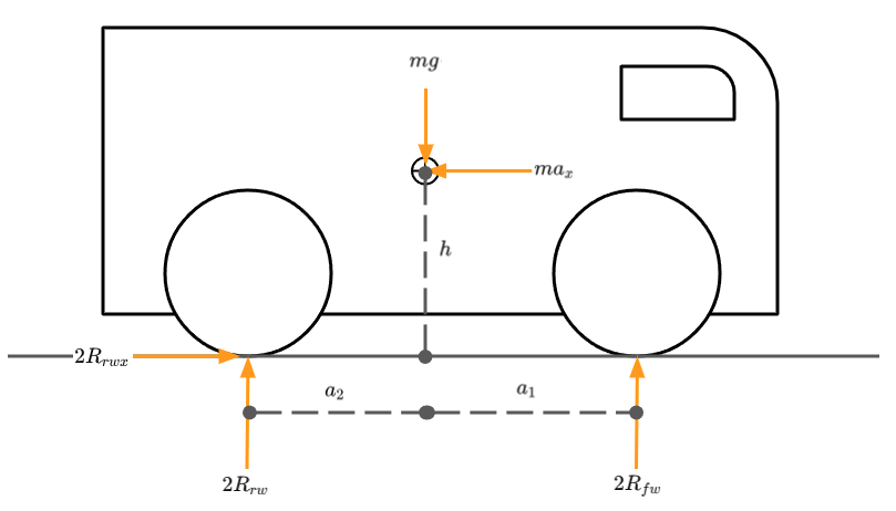
Figure 1: Level Ground Side View Free Body Diagram

The vehicle’s wheelbase can be defined as \(l\) as shown in equation (2). \[\begin{equation} l = a_1 + a_2 \tag{2} \end{equation}\]

Working in figure 1 we can apply the Newtonian laws of motion to this free body problem.

Working in the \(x\) direction. \[\begin{equation} \sum F_x = 0 \tag{3} \end{equation}\]

\[\begin{equation} \sum F_x = 2R_{rwx} - ma_x = 0 \tag{4} \end{equation}\]

Working in the \(z\) direction. \[\begin{equation} \sum F_z = 0 \tag{5} \end{equation}\]

\[\begin{equation} \sum F_z = mg - 2R_{rw} - 2R_{fw} = 0 \tag{6} \end{equation}\]

Summing moments at the centre of gravity about the \(y\) axis. \[\begin{equation} \sum M_{yy} = 0 \tag{7} \end{equation}\]

\[\begin{equation} \sum M_{yy} = 2 a_2 R_{rw} - 2 h R_{rwx} - 2 a_1 R_{fw} = 0 \tag{8} \end{equation}\]

Or at the rear wheel contact patch.

\[\begin{equation} \sum M_{yy} = a_2 m g - 2 l R_{fw} - h m a_x = 0 \tag{9} \end{equation}\]

Taking the above equations, we can then solve for our three unknown reactions \(R_{fw}\), \(R_{rw}\) and \(R_{rwx}\). Doing so yields equations (10), (11) and (12).

\[\begin{equation} R_{rwx} = \frac {1}{2} ma_x \tag{10} \end{equation}\]

\[\begin{equation} R_{fw} = \frac {1}{2} mg \frac {a_2}{l} - \frac {1}{2} ma_x \frac {h}{l} \tag{11} \end{equation}\]

\[\begin{equation} R_{rw} = \frac {1}{2} mg \frac {a_1}{l} + \frac {1}{2} ma_x \frac {h}{l} \tag{12} \end{equation}\]

When our ground vehicle is not accelerating, \(a_x\) equals zero, the conditions are met for static equilibrium. This results in equations (11) and (12) breaking into two parts. A static contribution, either \(\frac {1}{2} mg \frac {a_1}{l}\) or \(\frac {1}{2} mg \frac {a_2}{l}\), and a dynamic contribution \(\frac {1}{2} ma_x \frac {h}{l}\).

Level Ground Front View

The exact same process is applicable for the front view, \(yz\) plane, of the vehicle. Figure 2 shows our vehicle driving forwards towards the viewer. We are defining \(y\) right for the vehicle as positive (left in the image), \(z\) down as positive and moments about the \(x\) axis counter-clockwise positive.

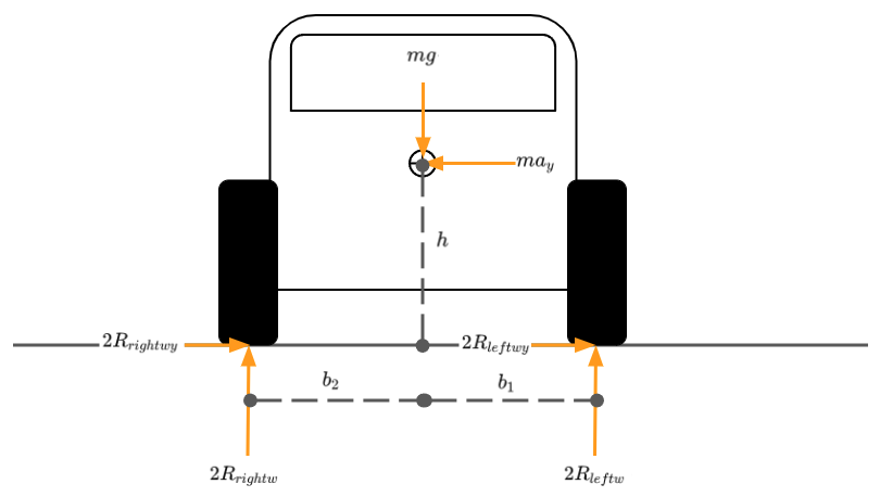
Figure 2: Level Ground Front View Free Body Diagram

The vehicle’s track can be defined as \(t\) as shown in equation (13). \[\begin{equation} t = b_1 + b_2 \tag{13} \end{equation}\]

Working in figure 2 we can apply the Newtonian laws of motion to this free body problem.

Working in the \(y\) direction. \[\begin{equation} \sum F_y = 0 \tag{14} \end{equation}\]

\[\begin{equation} \sum F_y = ma_y - 2R_{leftwy} - 2R_{rightwy} \tag{15} \end{equation}\]

Working in the \(z\) direction. \[\begin{equation} \sum F_z = 0 \tag{16} \end{equation}\]

\[\begin{equation} \sum F_z = mg - 2R_{leftw} - 2R_{rightw} \tag{17} \end{equation}\]

Summing moments at the centre of gravity about the \(x\) axis. \[\begin{equation} \sum M_{xx} = 0 \tag{18} \end{equation}\]

\[\begin{equation} \sum M_{xx} = 2 h (R_{leftw} + R_{rightw}) + 2 b_1 R_{leftw} - 2 b_2 R_{rightw} = 0 \tag{19} \end{equation}\]

Summing moments at the right contact patch. \[\begin{equation} \sum M_{xx} = ma_y h - m_g b_2 + 2 R_{leftw} = 0 \tag{20} \end{equation}\]

Taking the above equations we can return normal force contributions for the wheels on the left and right sides of the vehicle. \[\begin{equation} R_{leftw} = \frac {1}{2} mg \frac {b_2}{t} - \frac {1}{2} ma_y \frac {h}{t} \tag{21} \end{equation}\]

\[\begin{equation} R_{rightw} = \frac {1}{2} mg \frac {b_1}{t} + \frac {1}{2} ma_y \frac {h}{t} \tag{22} \end{equation}\]

As with the side view case these equations can be split into their static contribution \(\frac {1}{2} mg \frac {b_1}{t}\) or \(\frac {1}{2} mg \frac {b_2}{t}\) and dynamic contribution \(\frac {1}{2} ma_y \frac {h}{t}\).

Ascending Incline

We can take the case depicted in figure 1 and model the effect of the vehicle ascending an inclination. This is shown in figure 3.

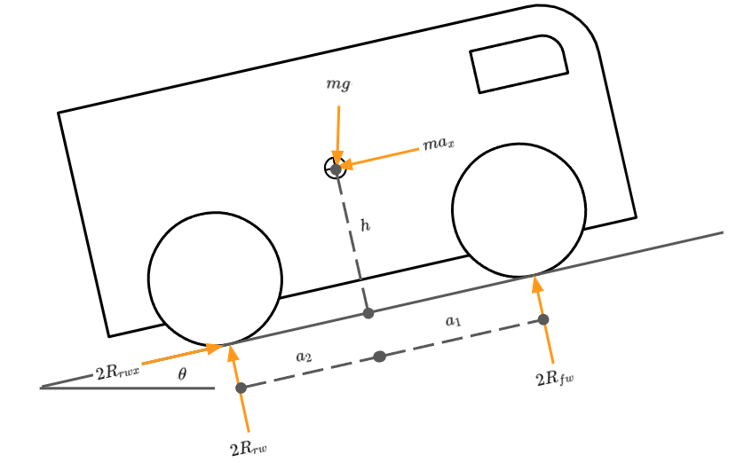
Figure 3: Incline Side View Free Body Diagram

\[\begin{equation} R_{fw} = \frac {1}{2} mg (cos \theta \frac {a_2}{l} - sin \theta \frac {h}{l}) - \frac {1}{2} ma_x \frac {h}{l} \tag{23} \end{equation}\]

\[\begin{equation} R_{rw} = \frac {1}{2} mg (cos \theta \frac {a_1}{l} + sin \theta \frac {h}{l}) + \frac {1}{2} ma_x \frac {h}{l} \tag{24} \end{equation}\]

\[\begin{equation} R_{rwx} = \frac {1}{2} mg sin \theta \tag{25} \end{equation}\]

Traversing Incline

Similarly to the previous scenario, we can take the case depicted in figure 2 and model the effect of the vehicle traversing along an inclination. This is shown in figure 4.

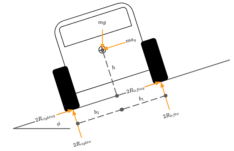
Figure 4: Incline Front View Free Body Diagram

\[\begin{equation} R_{leftw} = \frac {1}{2} mg (cos \phi \frac {b_2}{t} - sin \phi \frac {h}{t}) - \frac {1}{2} ma_y \frac {h}{t} \tag{26} \end{equation}\]

\[\begin{equation} R_{rightw} = \frac {1}{2} mg (cos \phi \frac {b_1}{t} + sin \phi \frac {h}{t}) + \frac {1}{2} ma_y \frac {h}{t} \tag{27} \end{equation}\]

Real Vehicle Design Validation

I’ll now present a simple method for validating that our design intent is what we have present in our real ground vehicle. This method is useful for prototype design validation, production design validation or even reverse engineering other vehicles.

Tilting Angles

Given the centre of mass position it is possible to determine the angles at which a ground vehicle would roll over. This condition occurs when the gravity vector falls outside of the polygon drawn by the contact patches of the vehicle’s wheels.

\[\begin{equation} \theta_{t_{front}} = atan(\frac {a_1}{h}) \tag{30} \end{equation}\]

\[\begin{equation} \theta_{t_{rear}} = atan(\frac {a_2}{h}) \tag{31} \end{equation}\]

\[\begin{equation} \theta_{t_{left}} = atan(\frac {b_1}{h}) \tag{32} \end{equation}\]

\[\begin{equation} \theta_{t_{right}} = atan(\frac {b_2}{h}) \tag{33} \end{equation}\]

Maximum Operable Incline

Whereas the tilting angles previously shown provide when the vehicle will roll over, in most real cases a vehicle will slide before it rolls. We can determine the angles at which the vehicle will begin to slide if we have an estimate for the friction coefficient between the vehicle’s wheels and the ground surface.

Assuming drive and breaking occur at the rear wheels only.

Ascending an incline \[\begin{equation} \theta = acot ( \frac {l}{\mu a_1} - \frac {h}{a_1}) \end{equation}\]

Descending an incline \[\begin{equation} \theta = acot ( \frac {l}{- \mu a_1} - \frac {h}{a_1}) \end{equation}\]

Modelling the Complex Case

Python Implementation

Let’s start by importing Numpy and defining some functions. I’ve short handed several trigonometric functions for brevity. I have also created two custom functions, one which compiles a 3D rotation matrix from Euler angles, and a second function that takes a slopes inclination and the attack angle of the vehicle to that inclination and returns the vehicle’s pitch and roll angles.

import numpy as np

# Short handing trig functions
sin = np.sin
cos = np.cos
tan = np.tan
asin = np.arcsin
acos = np.arccos
atan = np.arctan
atan2 = np.arctan2
pi = np.pi
to_rads = pi/180
to_degs = 180/pi


def cot(angle):
    """Calculate the cotangent of an angle
    """
    out = 1/tan(angle)
    return out


def acot(angle):
    """Calculate the arc cotangent of an angle
    """
    out = atan(1/angle)
    return out


def hpr2mat_parent2child(hea, pit, rol):
    '''Takes three Euler angles and returns a parent
       to child frame rotation matrix
    '''
    ca = np.array([[cos(hea*to_rads), -sin(hea*to_rads), 0],
                    [sin(hea*to_rads), cos(hea*to_rads), 0],
                    [0, 0, 1]])
    
    cb = np.array([[cos(pit*to_rads), 0, sin(pit*to_rads)],
                    [0, 1, 0],
                    [-sin(pit*to_rads), 0, cos(pit*to_rads)]])
        
    cc = np.array([[1, 0, 0],
                   [0, cos(rol*to_rads), -sin(rol*to_rads)],
                   [0, sin(rol*to_rads), cos(rol*to_rads)]])
    
    if hea != 0 and pit == 0 and rol == 0:
        return ca
    
    if hea == 0 and pit != 0 and rol == 0:
        return cb
    
    if hea == 0 and pit == 0 and rol != 0:
        return cc
    
    rot = ca @ cb @ cc
    
    rot = np.linalg.inv(rot)
    
    return rot


def calculate_orientation(attack_angle, incline):
    '''Takes an attack angle and inclination angle and
       returns vehcile pitch and roll angles
    '''
    compound_rot = hpr2mat_parent2child(attack_angle, incline, 0)
    
    x_unit = np.array([1, 0, 0])
    y_unit = np.array([0, 1, 0])
    
    x_rot = compound_rot @ x_unit
    x_rot_proj = np.array([x_rot[0], x_rot[1], 0])
    
    y_rot = compound_rot @ y_unit
    y_rot_proj = np.array([y_rot[0], y_rot[1], 0])
    
    pitch = acos((x_rot.T @ x_rot_proj) / (np.linalg.norm(x_rot) * np.linalg.norm(x_rot_proj))) * to_degs
    roll = acos((y_rot.T @ y_rot_proj) / (np.linalg.norm(y_rot) * np.linalg.norm(y_rot_proj))) * to_degs
    
    return pitch, roll

Next we can call these functions in order to establish the pitch and roll of the vehicle on a given incline.

attack_angle = 45
incline = 5

pitch, roll = calculate_orientation(attack_angle, incline)

Here I have given an attack angle of 45 degrees and an incline angle of 5 degrees, which results in a vehicle pitch of 3.533 degrees and a roll of 3.533 degrees.

Now we can specify all of our vehicle’s key parameters, the variable names ought to match those mentioned earlier in this post for clarity.

# Vehicle parameters
m = 40 # kg

# Vehicle CoG longitudinal position
a_1 = 0.4 # m
a_2 = 0.3 # m
l = a_1 + a_2

# Vehicle CoG lateral position
b_1 = 0.9/2 # m
b_2 = 0.9/2 # m
t = b_1 + b_2

# Vehicle CoG vertical position
h = 0.4 # m

# Proportion of Lateral Weight Transfer at the Front of the Vehicle
rho_mf = 0.5

# Friction Coefficient
mu = 0.6

We also need to add the dynamic boundary conditions and accelerations present at the given moment in time we wish to model.

# Dynamic conditions
g = 9.81 # m^2 / s

forward_speed = 0.4 # m / s
corner_radius = 15 # m | Positive for turning left

a_x = 3 # m^2 / s | Positive for forward acceleration
a_y = forward_speed**2 / corner_radius # m^2 / s | Positive for turning left

# Compute tilting Angles
theta_t_front = round(atan2(a_1, h) * to_degs, 2)
theta_t_rear = round(atan2(a_2, h) * to_degs, 2)
theta_t_left = round(atan2(b_1, h) * to_degs, 2)
theta_t_right = round(atan2(b_2, h) * to_degs, 2)

# Compute the maximum operable inclines before slipping
max_asc_angle = round(acot(l/(mu * a_1) - h/a_1) * to_degs, 2)
max_des_angle = round(acot(l/(-mu * a_1) - h/a_1) * to_degs, 2)

# TODO: add max traversing angle


# Debug values
static_front_axle = m * g * (cos(pitch) * a_2 / l - sin(pitch) * h / l)
static_rear_axle = m * g * (cos(pitch) * a_1 / l + sin(pitch) * h / l)

static_left_side = m * g * (cos(roll) * b_2 / t - sin(roll) * h / t)
static_right_side = m * g * (cos(roll) * b_1 / t + sin(roll) * h / t)

dynamic_longitudinal_transfer = m * a_x * h / l
dynamic_lateral_transfer = m * a_y * h / t

Now we can compute the normal forces under all four wheels and the subsequent masses that you might measure if you could put scales under those wheels.

# Compute reaction forces
R_fl = m * g * (cos(pitch) * a_2 / l - sin(pitch) * h / l) * (cos(roll) * b_2 / t - sin(roll) * h / t) - 1/2 * m * a_x * h / l - rho_mf * m * a_y * h / t
R_fr = m * g * (cos(pitch) * a_2 / l - sin(pitch) * h / l) * (cos(roll) * b_1 / t + sin(roll) * h / t) - 1/2 * m * a_x * h / l + rho_mf * m * a_y * h / t
R_rl = m * g * (cos(pitch) * a_1 / l + sin(pitch) * h / l) * (cos(roll) * b_2 / t - sin(roll) * h / t) + 1/2 * m * a_x * h / l - (1 - rho_mf) * m * a_y * h / t
R_rr = m * g * (cos(pitch) * a_1 / l + sin(pitch) * h / l) * (cos(roll) * b_1 / t + sin(roll) * h / t) + 1/2 * m * a_x * h / l + (1 - rho_mf) * m * a_y * h / t

R_fl = round(R_fl, 3)
R_fr = round(R_fr, 3)
R_rl = round(R_rl, 3)
R_rr = round(R_rr, 3)

# Compute corner weights
m_fl = round(R_fl / g, 3)
m_fr = round(R_fr / g, 3)
m_rl = round(R_rl / g, 3)
m_rr = round(R_rr / g, 3)

Our inputs for the vehicle and conditions yield the following…

Static Conditions | Pitch (\(\theta\)) = 3.533 degrees | Roll (\(\phi\)) = 3.533 degrees

Dynamic Conditions | Forward Acceleration (\(a_x\)) = 3 \(m/s^2\) | Lateral Acceleration (\(a_y\)) = 0.0106667 \(m/s^2\)

Under the Front Left Wheel | Mass = 3.901 kg | Normal Force = 38.271 N

Under the Front Right Wheel | Mass = 4.781 kg | Normal Force = 46.898 N

Under the Rear Left Wheel | Mass = 14.91 kg | Normal Force = 146.267 N

Under the Rear Right Wheel | Mass = 16.256 kg | Normal Force = 159.474 N

Sum of Calculated Masses = 39.848 kg | Original Mass = 40 kg

Found this useful or interesting?

Surely after all this I deserve a drink?! Consider donating to support.

Any question, comments, corrections or suggestions?

Reach out on the social links below through the buttons.