Ground Vehicle Centre of Mass Optimisation
Preamble
In a previous post on Weight Distribution in Mobile Ground Vehicles I provided a model for determining the forces able to be generated by a ground vehicle, which ultimately will be a limiting factor in performance. I also provided a method for establishing the centre of mass location of a ground vehicle, providing that you have one to start with.
If you are at an earlier stage in design you may not have a ground vehicle to analyse and want to get a good estimate for the centre of mass location prior to manufacturing your first prototype. This post will look to present a simple model that can be used to estimate some of the key parameters needed much more quickly than modeling your prototype accurately in CAD.
Approach
We’ll use a lumped mass model of our vehicle’s sub-systems. Knowing the approximate mass budget for each sub-system and the approximate position of that sub-system’s centre of mass in the vehicle we can then calculate where the centre of mass for the complete vehicle will be. This method can produce good results providing you included all the sub-systems with a significant contribution.
Lumped Mass Model
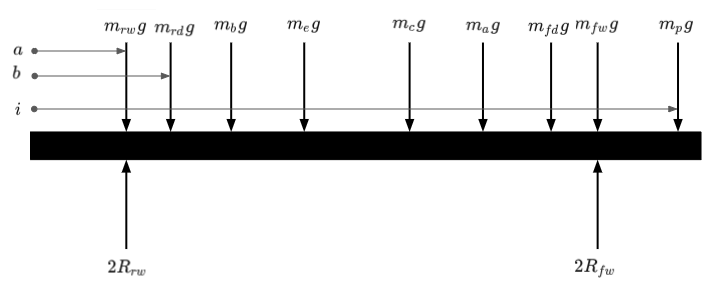
For demonstration purposes I’ve assumed a four wheeled ground vehicle with all four wheels being driven. It is equipped with electric drive, a battery, a perception senor suite and some actuators to do work. Within some bounds we will often have the freedom to move these sub-systems around in order to optimise the centre of mass location of the vehicle. We can approximate our ground vehicle as a beam with masses applied to it from the separate functional sub-systems with the most significant mass contributions. Working in this way we can establish what the reactions at the wheels are, then where the vehicle’s centre of mass location is.
The table below details the sub-systems and their location in the vehicle.
| Sub-System | Force Contribution | Distance From Rear |
|---|---|---|
| Rear Wheels | \(m_{rw} g\) | \(a\) |
| Rear Drives | \(m_{rd} g\) | \(b\) |
| Battery | \(m_b g\) | \(c\) |
| Electronics | \(m_e g\) | \(d\) |
| Chassis | \(m_c g\) | \(e\) |
| Actuators | \(m_a g\) | \(f\) |
| Front Drives | \(m_{fd} g\) | \(g\) |
| Front Wheels | \(m_{fw} g\) | \(h\) |
| Perception | \(m_p g\) | \(i\) |
| Total | \(m_{tot}g\) | \(j\) |
A side view (\(xz\) plane) of the vehicle with locations of mass contributions is shown in figure 1. Note that some of the distance labels have been omitted for the clarity of the diagram. You will also note the reaction forces under each of the front wheels, \(R_{fw}\), and each of the rear wheels, \(R_{rw}\).
The total mass of our ground vehicle, \(m_{tot}\), ought to be the sum of all of the mass contributions of the sub-systems, equation (1).
\[\begin{equation} m_{tot} = m_{rw} + m_{rd} + m_b + m_e + m_c + m_a + m_{fd} + m_{fw} + m_p \tag{1} \end{equation}\]
If we call the vertical \(z\) axis and applying static equilibrium whilst summing forces yields the following.
\[\begin{equation} \sum F_z = 0 \tag{2} \end{equation}\]
\[\begin{equation} \sum F_z = (m_{rw} + m_{rd} + m_b + m_e + m_c + m_a + m_{fd} + m_{fw} + m_p)g - 2R_{rw} - 2R_{fw} \tag{3} \end{equation}\]
\[\begin{equation} R_{fw} = \frac {(m_{rw} + m_{rd} + m_b + m_e + m_c + m_a + m_{fd} + m_{fw} + m_p)g - 2R_{rw}}{2} \tag{4} \end{equation}\]
\[\begin{equation} R_{rw} = \frac {(m_{rw} + m_{rd} + m_b + m_e + m_c + m_a + m_{fd} + m_{fw} + m_p)g - 2R_{fw}}{2} \tag{5} \end{equation}\]
Now if we sum moments under equilibrium at the front wheel we can derive an expression for \(R_{rw}\). Note that clockwise rotation is positive.
\[\begin{equation} \sum M_{yy} = 0 \tag{6} \end{equation}\]
\[\begin{equation} \sum M_{yy} = (h-a)2R_{rw} - (h-a)m_{rw}g - (h-b)m_{rd}g - (h-c)m_bg - (h-d)m_eg - (h-e)m_cg - (h-f)m_ag - (h-g)m_{fd}g + (i-h)m_pg \tag{7} \end{equation}\]
\[\begin{equation} R_{rw} = \frac {g((h-a)m_{rw} + (h-b)m_{rd} + (h-c)m_b + (h-d)m_e + (h-e)m_c + (h-f)m_a + (h-g)m_{fd} - (i-h)m_p)}{2(h-a)} \tag{8} \end{equation}\]
Once we have \(R_{rw}\) we can use equation (4) to provide \(R_{fw}\). The corner weights we could expect under each wheel can be given using equation (9) and (10).
\[\begin{equation} m_f = R_{fw}g \tag{9} \end{equation}\]
\[\begin{equation} m_r = R_{rw}g \tag{10} \end{equation}\]
Now we can calculate the vehicle’s centre of mass location, \(j\), with respect to the front wheel location, \(h\), in equation (11).
\[\begin{equation} h-j = \frac {l}{m_{tot}} 2 m_r \tag{11} \end{equation}\]
Similarly the centre of mass location, \(j\), with respect to the rear wheel location, \(a\), is provided with equation (12).
\[\begin{equation} j-a = \frac {l}{m_{tot}} 2 m_f \tag{12} \end{equation}\]
A useful simple check that can be done is to check the wheelbase, \(l\), of the vehicle against the sum of the results from equations (11) and (12).
\[\begin{equation} l = h-a \tag{13} \end{equation}\]
\[\begin{equation} (h-j) + (j-a) = l \tag{14} \end{equation}\]
Wrap Up
In the example shown here we have only were in the vehicle’s longitudinal plane, but it’s easy to apply this also the to vehicle’s lateral plane to establish the 2D centre of mass location.
Hopefully you can see how using the method presented here along with the model given in Weight Distribution in Mobile Ground Vehicles to quickly get to a performant ground vehicle. You can also use the validation method from the other post to see how well you estimated these parameters.
Hey you!
Found this useful or interesting?
Consider donating to support.
Any question, comments, corrections or suggestions?
Reach out on the social links below through the buttons.