A GNSS Primer for Roboticists
Preamble
Global Navigation Satellite System (GNSS) is a generic term that encompasses several satellite based positioning systems (GPS, GLONASS, GALILEO, BEIDOU and QZSS). This post is intended to provide a broad background on how GNSS works for those integrating or using GNSS as part of their own platforms, to ensure they are armed with enough information to make good decisions when setting up systems and hopefully avoid some of the common pitfalls. As such this article is well suited to engineers across several disciplines and sectors due to the pervasiveness of GNSS technologies.
Constellations
Here is a quick run down of the different constellations:
- GPS (USA)
- 24 satellites plus 8 spares
- 55 degree inclination from the equator and ~12 hour orbital period
- All use the same frequency with unique PRNs
- L1 carrier frequency of 1575.42 MHz
- L2 carrier frequency of 1227.6 MHz
- GLONASS (Russia)
- 24 satellites plus spares
- three separate distinct orbital planes, each with 6 satellites and ~11 hour orbital period
- All use the same “PRN” with a unique frequency
- L1 carrier frequency of 1598-1609 MHz
- L2 carrier frequency of 1243-1252 MHz
- GALILEO (Europe)
- Ideally 24 satellites plus 6 spares
- Currently 23 usable satellites and 5 down, at time of writing
- 56 degree inclination from the equator and ~14 hour orbital period
- All use the same frequency with unique PRNs
- L1 carrier frequency of 1575.42 MHz
- L2 carrier frequency of 1246 MHz
- BEIDOU (China)
- Complicated due to having three phases of operation, take a look at the Wiki
- QZSS (Japan)
- Again, I’d recommend the Wiki here so you can take a look at the interesting orbital path visualisations
When looking at GNSS hardware, broadly speaking, the more constellations your receiver uses the more resilient you will be to poor sky view and satellite loss. You won’t necessarily be “more accurate” but you will likely be accurate more of the time. Think of additional constellations as providing margin for error in difficult conditions, as you have more satellites available to use to calculate a solution.
How it Works
Each constellation is generally made up of three parts:
- Space Segment - satellites on orbit, transmitting Almanac, Ephemeris and Pseudo-Random Noise (PRN)
- Control Segment - ground control stations that take care of the orbital models, timing offsets, etc.
- User Segment - receivers and antennas
The basic concept is that given that a signal travels from the satellite at the speed of light, \(C\). If we know how long that signal took to reach us, \(t\), then we can calculate our distance, \(d\), to each satellite.
\[\begin{equation} d = C \times\ t \end{equation}\]
Timing here needs to be incredibly accurate. Given that the speed of light is a very large number, 299,792,458 m/s, small errors in timing measurements will have a large effect on the distance. In order to even get to metre level positioning accuracy, timing accuracy needs to be of the order of tens of nanoseconds or 1e-8 seconds. This, indeed, is one of the bonuses of using GNSS hardware in your robotics platforms, you get a very accurate timing source for “free”.
In order to find the position of the user hardware we need at least four satellite observations for the simplest solution. This allows us to setup a system of four simultaneous equations, solving for three dimensional positions (x, y, z) and time (t).
Real Time Kinematic (RTK) Solutions
RTK is where things get interesting, as this is where we can get down to centimeter level accuracy. RTK attempts to calculate the exact number of wavelengths between the satellites and the antenna of a fixed reference station in an attempt to provide either an RTK float or RTK integer solution. This process is known as ambiguity resolution. RTK integer solutions utilise an algorithm that will only yield a whole number of wavelengths, whereas an RTK float solution will allow for decimals. Typically RTK float is only used as a fallback solution in situations where an RTK integer solution cannot be found.
There are several considerations when implementing an RTK system:
- The absolute geographic accuracy of your system will depend on the accuracy of the base station location used for corrections, more on this here. If this reference station moves your rovers position will also move by the same amount unless the reference station’s location is reset. This can be an issue in some cases but I have also found it to be a benefit in others.
- Requirement for fixed local reference stations and communication infrastructure between rover and fixed station, or logging and post processing. If you are going to take on the cost and maintenance of this infrastructure then you should spend some time considering what the long term impacts of that will be.
- Accuracy typically falls off at a rate of around 1 PPM as a function of the distance between the rover and the local reference station. ie. 1 cm of accuracy is lost for every 10 km of distance.
- If you are utilising a commercial correction service (usually through an NTRIP provider) you will need a two way data connection in order to provide the service with an approximate location of your rover for matching with the nearest local reference station.
- There must be inter visibility of satellites between reference station and rover. As six satellites are required for an RTK solution this means that the same six usable satellites must be observable for the reference station and the rover at the same time, so make sure your reference station(s) have the best sky view possible if you are self managing these.
Accuracy, Precision and Repeatability
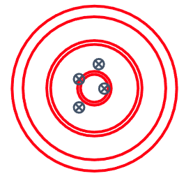
When talking about any localisation methods, accuracy is always one of the first questions to come up. However, it is very important to define terms and metrics before quoting any values, in order to avoid confusion and disappointment. Accuracy is typically considered as how close you are able to measure to the true value of something. Precision and repeatability are measures for how well the measurement results can be repeated and the variability of those repeated measurements.
Get ready for the classic depiction using the clustering of shots on a target…
| Target Representation | Accuracy | Precision |
|---|---|---|
 |
High Accuracy | High Precision |
 |
High Accuracy | Low Precision |
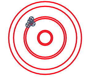 |
Low Accuracy | High Precision |
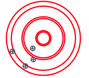 |
Low Accuracy | Low Precision |
Absolute Geographic Accuracy vs. Other Forms of Accuracy
Typically I find that localisation solutions are required to be accurate to different reference true values, dependent on application.
It may be the case that you need absolute geographic accuracy to an existing datum so that you can incorporate external data sources, or have your data easily used by others.
Alternatively, maybe you need repeatable results, such that your rover always returns to the same place on repeated runs, but have no care for absolute geographic accuracy.
Another case might be that you have some other datum you need to be accurate against such as an independently sourced map or image.
In all three cases a high level of repeatability and accuracy is called for but the true value that we need to be accurate to has altered.
When operating using RTK position solutions we should take care with our reference station positions, as this is ultimately our shot on target. In this way it is better to think of RTK as providing centimetre level precision and repeatability, which could be accuracy too, depending on how well setup your local reference station is. If we are self-managing our base stations then it is up to us to decide what we want to be accurate to and how we are going to go about achieving this.
Accuracy Metrics
Circular Error Probable (CEP) is often the method used to quantify GNSS positioning errors. Typically we quote to a 50% CEP, ie. 50% of our observations fall within a circle of a given radius. If a receiver was reporting an accuracy of 0.8 m CEP then 50% of it’s observations would fall within a circle of radius 0.8 m. Another way to think of this is that the receiver will be within 0.8 m of the true measurement 50% of the time.
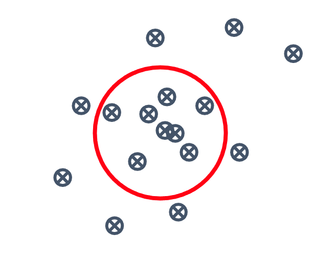
Figure 1: Circular Error Probable
An alternative, but often used approach is to utilise Root Mean Square Error (RMSE), where we take the square root of the average of the squared errors, typically quoted to one standard deviation (providing the mean is zero).
Dilution of Precision (DOP) is a measure of how well spaced the satellites that are currently being used in the localisation solution are. High values of DOP means that the satellites being utilised are close together in the sky, figure 2.
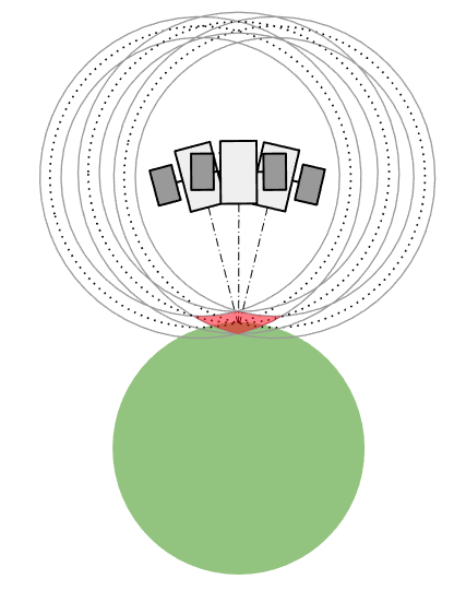
Figure 2: Poorly Spaced Satellites Yielding Poor DOP
This then leads to a less accurate solution than if the satellites being utilised were well spaced, figure 3.
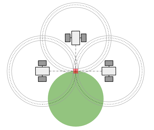
Figure 3: Well Spaced Satellites Providing Good DOP
Note that poor DOP usually comes as a result of ground level obstructions blocking the view of satellites that could have been utilised otherwise.
Resolution
When dealing with global frame coordinates, latitudes and longitudes, in decimal degrees you need to take care in preserving resolution across any stages in your processing. The number of decimal places used and your approximate latitude have an interplay that will effect the 2D positional accuracy you are able to achieve.
The data provided below is calculated based on the WGS84 model. It shows how variation of resolution effects differences in position, for a selection of latitudes. Northing and Easting here, being 2D components of position on the ground and have been combined to provide the 2D accuracy possible for each scenario.
For most applications utilising RTK integer solutions and centimetre level positioning eight or nine decimal places should provide enough head room.
An Intentionally Brief Word on Geodetic Models and Datums
When we are looking at accuracy it is worth taking some time to be sure that we are aware of what reference system we are measuring in, especially when comparing data from multiple sources. Most of the time these are configurable in your GNSS receiver, so it ought to be a case of selecting the one you need for your application, unless you are utilising a third party correction source. If this is the case then your end localisation solution will be in the datum of the correction source used. For the most part people have generally settled on WGS84 at the time of writing, however, NAD83 is still fairly pervasive in the USA so just take care, especially when using NTRIP providers.
- International - WGS84, ITRF00, ITRF 08
- USA - NAD83 - State plane system
- Europe - ETRS89
- UK - OSGB36
Solution Types
Standard Positioning Service
- Minimum Number of Satellites: Four (x, y, z, t)
- Expected Accuracy: ~1.5 m CEP
Differential GNSS
- Minimum Number of Satellites: Four (x, y, z, t)
- Expected Accuracy: ~45 cm CEP
- Differential Method: Code Phase
RTK Float
- Minimum Number of Satellites: Six (x, y, z, t, L1, L2)
- Expected Accuracy: ~20 cm CEP
- Differential Method: Carrier Phase
- Wavelength Ambiguity: Floating Point
RTK Integer
- Minimum Number of Satellites: Six (x, y, z, t, L1, L2)
- Expected Accuracy: ~1-2 cm CEP
- Differential Method: Carrier Phase
- Wavelength Ambiguity: Integer
Free Satellite Based Augementation Services (SBAS) - WAAS/ EGNOS/ MSAS/ GAGAN
- Minimum Number of Satellites: Six (x, y, z, t)
- Expected Accuracy: ~60-100 cm CEP
- Typically only contains corrections for GPS satellites
- Data not available worldwide
- Does not correct for local atmospheric and ionospheric conditions
Paid For Satellite Based Correction Services - Omnistar, Terrastar
- Minimum Number of Satellites: Six (x, y, z, t, L1, L2)
- Expected Accuracy: ~10 cm CEP
- Worldwide data
- Does not correct for local atmospheric and ionospheric conditions
Sources of GNSS Errors
Atmospheric and Ionospheric
Noise and delays due to having the GNSS signal travel through the atmosphere and ionosphere. As we are trying to estimate our position based on the time of flight for the GNSS signals, if the signal takes longer to reach us then our position will be inaccurate. However, these are typically constant over a given ground location and can be mitigated using RTK solutions.
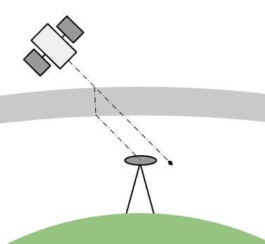
Figure 4: GNSS Error Induced by Atmospheric and Ionospheric Conditions
Space Segment Error
If the space segment is reporting satellite positions or time stamps incorrectly then this error will propogate into errors with the position solutions in the ground segment. Much like the atmospheric and ionospheric errors, these are typically constant over a given ground location and can be mitigated using RTK solutions.
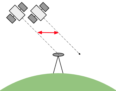
Figure 5: GNSS Error Due to Space Segment Errors
Multipath Reflections
Where the GNSS signal is reflected through an alternative path to the antenna. The alternate path will have a different time of flight and thus will cause position errors. Unlike the previous two error sources, these vary with the rovers pose, the surrounding environment and time, due to the changing geometry of the available GNSS satellites.
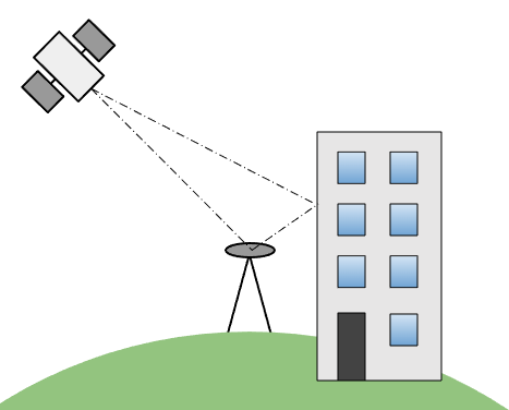
Figure 6: GNSS Error Due to Multipath Reflections
Other Considerations
Antenna Selection
Generally antennas will come in an OEM style, without a radome cover and with a radome cover. Keep in mind that an antenna with a plastic radome cover will often have a different tuning to account for the radome versus it’s OEM style equivalent. If your application has it’s own outer cover it’s worth considering getting in touch with an antenna manufacturer to see if they can create a custom tuning for one of their OEM style antennas to work with your integrated cover. I know that this is a service that Tallysman used to offer, as well as several other manufacturers, I’m sure.
Broadly speaking, I would always try to utilise active antennas over passive ones, ideally with LNA gain greater than 17 dB. Built in multipath signal rejection and carrier phase linearity are good things to look out for when selecting antennas.
Antennas with a SAW filter can be utilised in environments where LTE or WiFi signals may cause some interference.
Below are a selection of antennas I have used in the past with good results, however, your selection will depend on how the antenna pairs with your GNSS receiver.
Ground Planes
A ground plane is a piece of material which is designed to block multipath reflections coming up from below the antenna. The material selection should be one that suits your application but it must block RF signals as much as is feasible.
The geometry of the ground plane is typically a thin disk. The diameter ought to be at least a half of the wavelength of the radio waves the antenna is receiving. L1 GNSS frequencies are ~1575 MHz, with L2 being ~1227 MHz. This leads to a minimum sized ground plane having a diameter of ~10 cm.
Electromagnetic Interference (EMI) and Carrier to Noise Ratio (CNR)
An integral component to the performance of a GNSS system is the sensitivity to the GNSS signals of the antenna and receiver pair. Carrier to noise ratio (CNR) is a common metric reported by GNSS receivers to indicate the performance of the hardware. CNR is the ratio of carrier power to noise power, normalised across a 1 Hz bandwidth.
CNR testing can be utilised to evaluate different GNSS receivers, antennas, ground planes, radomes and even to detect local sources of electromagnetic interference (EMI) that would disrupt GNSS signals. It is an indispensable tool for system integrators.
Many receivers also reject satellites with CNR levels below a particular threshold, determining that there is too much noise to provide a reliable solution. Typical limits are around 30-35 dB-Hz for L1 and 20-25 dB-Hz for L2, these values often can also be altered by the user, but do so with caution as you may end up with a worse solution as a result.
There are multiple tests that can be employed depending on what variable you are looking to see the impact of. I will outline two strategies that should highlight how you might go about constructing a test for a given scenario, but the TLDR is:
- Log the CNR, usually through the NMEA GPGSV, GLGSV, GAGSV and GBGSV messages (constellation specific), and establish a base line reading
- Change the hardware setup or run multiple setups in parallel at the approximate same location
- Contrast the data recorded and make a judgment
Antenna Testing
- Setup your candidate antenna at least 0.5 m apart, with a clear unobstructed sky view
- Be sure to use appropriate ground planes where required
- If possible utilise multiple identical GNSS receivers, one for each antenna
- Ensure that firmware and configurations are identical across all receivers
- Begin recording the appropriate GSV messages from each receiver
- Plot the data and look for differences in CNR for specific satellites (identified by their PRN), between each candidate antenna. It’s usually best to focus on the best 3-5 satellites when doing this
An alternate tricky method can be employed if only one receiver is available, whereby each antenna is setup with the same cable and they are switched out, in turn, at the receiver. The receiver is left constantly on and outputting the CNR data to be logged. Keeping a record of the order and approximate times of the antenna swaps and correlating this to step changes in the CNR data will give a good indication of which antenna makes a better match to your receiver.
Integrated System EMI Testing
- Setup your platform with a clear unobstructed sky view
- Power on the minimum equipment required to boot the GNSS receiver
- Begin recording the appropriate GSV messages from your receiver
- Systematically power on each other aspect of your device, motors, cameras, etc. Be sure to keep a record of the order and approximate times that each of these events occurred
- Plot the data and look for step changes in CNR that coincide with one of these events. It’s usually best to focus on the best 3-5 satellites when doing this
- Consider ways to shield the GNSS equipment from the EMI caused by the worst offenders
Typical Results and Interpretation
I have provided a couple of example plots showing both time series CNR data, figure 7, and constellation positions, figure 8, as available from the NMEA GSV messages. When looking at these numbers it is important to keep in mind that dB-Hz is a logarithmic scale. Note that the observations that show up close to the horizon in figure 8 often have the lowest CNR (greatest noise) in figure 7. This is due to those signals typically traveling through more atmosphere and ionosphere due to there low elevation angle.
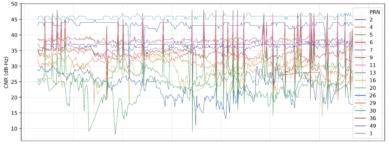
Figure 7: A Typical CNR Time Series Plot

Figure 8: A Typical Sky View Satellite Plot
When looking at the best three to five satellites from your data Tallysman say to interpret results in the following way “54dB is amazing, 53dB is excellent, 52dB is good and 49/50dB is ho-hum”. However, I imagine this is for a standalone GNSS receiver with a well tuned antenna, rather than a GNSS receiver integrated into a robotic platform or other vehicle, but this is still good for reference. Personally I have found that it is more reasonable to aim for 40-50 dB-Hz for L1 frequency signals and 35-40 dB-Hz for L2, but maybe I’m just “ho-hum” at doing this.
Communication Layer for Corrections
Serial radio modems are probably the most prolific method to transmit corrections from a self-managed local base station. These generally provide good range and reliability, however for many applications where other forms of connectivity are already available it often makes sense not to add the additional radio hardware.
For applications with data connections (WiFi, cellular, etc.) a software NTRIP (Network Transmission of RTCM over IP) client can be deployed, coupled with either a paid for subscription NTRIP service or self-managed NTRIP server connected to your own GNSS reference stations. The NTRIP protocol allows for two way communication between rovers and multiple base stations. This allows a rover to provide it’s approximate current location and request corrections from the station that is closest to it. NTRIP is worth investigating at if you are looking at working over very large areas (10+ km) or managing multiple base stations of your own.
Custom connections utilising TCP, UDP, DDS, MQTT, ZeroMQ, etc. for a communication transport layer, all make for fair alternatives to NTRIP, especially if you have local point to point connections, or some custom policies about which base stations you’d like rovers connect to. I have found that UDP provides the lowest latency and, given how reliable most modern networks are, packets are rarely dropped, and even when they are it typically isn’t an issue.
Correction packets can technically be considered as valid for as long as it the ionospheric and atmospheric conditions remain stable for, however, we generally have no idea if this is the case or not. As such, most GNSS receivers allow you to set a limit on how old a correction packet can be and still be utilised in it’s solution, this is often referred to as the “diff. age”. This value usually defaults to sixty second for most receivers. So if we are sending GNSS correction once every 2-10 seconds, we can afford to drop several packets before hitting this limit of sixty seconds. Ultimately you will need to do some testing and benchmarking of your connectivity to see what sort of frequencies and limits on diff. age make sense for your system.
Resources and Further Reading
Hey you!
Found this useful or interesting?
Consider donating to support.
Any question, comments, corrections or suggestions?
Reach out on the social links below through the buttons.